
RFC 3: Tiled and multiscale points#
RFC 3 · draft · data model; storage format · created 2026-09-17
Abstract#
Specification for spatially indexing points, enabling optional multiscale subsampled levels, spatially chunked storage: a regular 2-D or 3-D grid of tiles, with the points stored in tile-major order and, optionally, in feature-major order. Each point carries a random value \(p\), which defines the levels. This enables viewers and other processing applications to load only the points in view, or only those of the genes shown; zoomed out, they load a density-preserving sample, with as many points as the resources they have available allow (memory, bandwidth, rendering time). Shapes are in RFC 4.
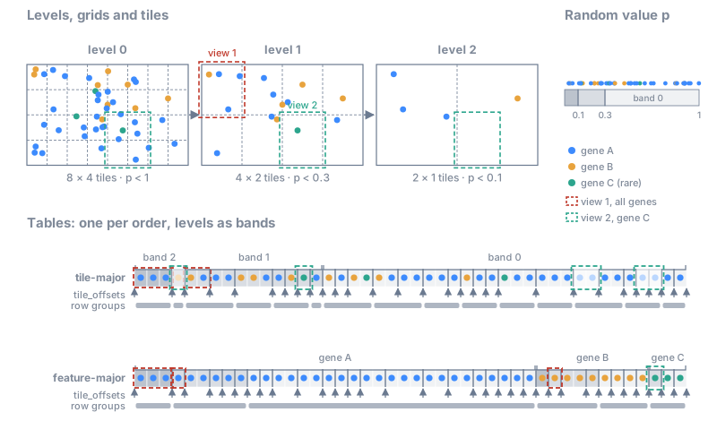
Overview of the spatial index; each part is described in the text.#
Description#
The key words MUST, MUST NOT, SHOULD, SHOULD NOT and MAY are to be interpreted as described in RFC 2119. Key words have this meaning only in capitals (RFC 8174).
Motivation#
Without an index, a reader can already skip the Parquet row groups whose minimum and maximum coordinates fall outside a box, and data written in spatially grouped row groups (as by the 10x Xenium and Atera software) then answer box queries quickly on a local disk: in a test with 1.2 billion transcripts, a 200 µm box kept 15% of the row groups and scanned 176 million rows to return 0.5 million points, in 0.2 s on a 14-core laptop with the data in memory. This does not hold remotely, where the same query reads gigabytes instead of the few megabytes of the tiles in view; it cannot sample, so a zoomed-out view reads every row group; and it cannot select features, unless the data happen to be sorted by feature. These are the cases the index is for.
Scope#
In scope: points, 2-D and 3-D; spatial indexing via chunking and sorting; tile-major order and feature-major order; sampled levels; a per-point random value \(p\).
Out of scope: shapes (RFC 4), the matrix of a table annotating the shapes and its sparse storage (CSR/CSC, RFC 4), aggregation to cells or bins (square/hexagonal), spatial orders inside tiles (Morton, Hilbert), ordering of the tiles other than C order (e.g. Morton).
Data model#
The data model does not depend on how the points are stored, in Parquet or in Zarr (Storage format).
Overview#
This section is an overview: it lists all the terms of the spatial index and how they relate. Each is defined in the sections that follow, starting from the tiles, then \(p\), which defines levels and bands on top of them; Summary lists them again in a table, with which are required. The terms are in three layers: the data, the data model and the storage format.
Data. The points with their columns (coordinates, feature, any other) are always there, as today. The data model and the storage format of the spatial index are optional: an element may have no spatial index at all. If it has one, some of its parts MUST be present, others SHOULD or MAY be.
Data model. It says which tile and which level each point belongs to:
grid parameters: the axes; per axis, the origin \(o_a\) and the tile size \(s_a\) of level 0; the grid of every coarser level, which refines the next one (recommended recipe: the merge rule) (Grid and tiles);
sampling parameters: a random value \(p\) per point, and the fraction \(P^{(l)}\) of each level, a fixed rate, by default the ratio of the tile volumes of level 0 and level \(l\) (\(1/2^d\) per level when all \(d\) axes are merged); level \(l\) holds the points with \(p < P^{(l)}\) (Priority, Levels and bands, Sampling);
derived from these, the number of points per tile at each level, which guides the choice of the tile size and the rates together (Choosing the tile size and the rates);
the feature column (e.g. the gene), which sorts the feature-major order (Tile-major order and feature-major order).
Storage format. It says how the points are written (Storage format), in Parquet or in Zarr:
the metadata declares which parts are present: the orders (tile-major and feature-major), the levels, and the grid and sampling of each level; in Parquet, a sidecar JSON file lists the part files of each table;
each order is one table, with the levels as bands of rows, with offsets that address rows:
tile_offsetsin the tile-major table (the tile index) and in each feature-major table (the feature index), and the column__spatialdata_p__, which stores \(p\); the row groups (Parquet) or chunks (Zarr) are a choice of the writer.
Grid and tiles#
A grid is defined for a specific points element (the SpatialData term for a 2D/3D points cloud), in the coordinates of its points. The metadata MUST specify the axes of the grid, and the grid MUST have all the spatial axes of the element; it MAY have a single tile along an axis, for instance along \(z\) for a thin section of tissue.
Each element has its own grid, chosen for its own data: two elements, for instance the transcripts and the cells of a dataset, do not have to share a grid (see RFC 4 for the shapes, which recommends nested grids when a client loads both tile by tile).
An axis \(a\) is one of the spatial axes \(x\), \(y\) and \(z\) (not the channel axis \(c\)). The grid has, per axis \(a\), an arbitrary origin \(o_a\), which MUST be given (for instance the corner with the minimum coordinates of the bounding box of all the points), one tile size \(s_a\), which MUST be given (square tiles are a special case), and an arbitrary number of tiles \(n_a\): the number of intervals into which the grid divides axis \(a\), not the total number of tiles of the grid, which is \(N = \prod_a n_a\). All the tiles are identical. The tiles MUST cover all the points. Each tile is to be interpreted as a semi-open hyper-interval, with the interval closed for the lowest value, and open for the highest. For example, in 2 dimensions, the tile
contains the points \((x, y)\) that satisfy \(x_{\min} \le x < x_{\max}\) and \(y_{\min} \le y < y_{\max}\).
The grid of every level present, \(0, \dots, L\), MUST be given in the metadata (see Metadata); since level 0 is always present, so is its grid. The grids of the coarser levels are the writer’s choice, with one constraint: the grid of each level \(l\) MUST refine the grid of level \(l + 1\), that is every tile of level \(l\) MUST lie inside a single tile of level \(l + 1\), so that no tile of a finer level overlaps several tiles of a coarser level. The grids SHOULD get coarser with the level, but a level MAY keep the grid of the level below, since a grid refines itself: at the limit, a single tile for the whole dataset at every level, or the same grid at all the levels, which avoids the many small, almost empty tiles of the coarse levels of a rare feature.
A recommended recipe, the merge rule, builds the grid of each coarser level from the grid of the previous level: it is merged by a factor of 2 along one or more axes, keeping the tiles as isotropic as possible. It satisfies the constraint, since the origin stays the same and each tile size is either kept or doubled, and the initial grid then determines the granularity of the spatial index at every level. Below are two merging steps that keep the tiles as isotropic as possible: in the first, by merging along one axis; in the second, by merging along two axes.
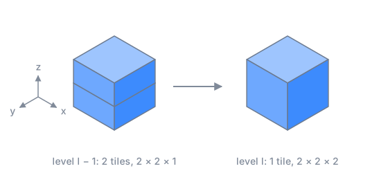
Merging along one axis (z). Tile sizes along (x, y, z).#
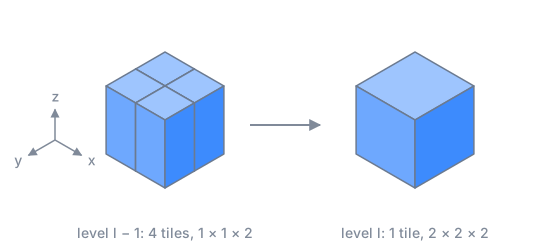
Merging along two axes (x and y). Tile sizes along (x, y, z).#
The rule in formulas
Let \(s_a^{(l)}\) and \(n_a^{(l)}\) be the tile size \(s_a\) and the number of tiles \(n_a\) along axis \(a\) at level \(l\). At level \(l\):
\(A^{(l)}\) are the axes that still have more than one tile at level \(l - 1\);
\(m^{(l)}\) is the smallest tile size among them;
\(M^{(l)}\) are the axes that will be merged at level \(l\): those of \(A^{(l)}\) whose tile size is less than twice \(m^{(l)}\).
Applied to the end, the merge rule stops at the first level with \(n_a = 1\) along every axis (a single tile). A writer may also stop earlier, so the lowest-resolution level may still contain multiple tiles.
Example: an anisotropic extent, 10 × 100 × 1000 along (z, y, x), origin 0.
Anisotropic tiles: initial tile size 1 × 10 × 100
Starting from “# tiles along axis” 10 × 10 × 10, the thin axes are merged first; z then stops at a single tile, and x is merged last:
level  tile size (z, y, x)  # tiles along axis (z, y, x)  merged
0         1 ×  10 ×  100    10 × 10 × 10                  -
1         2 ×  10 ×  100     5 × 10 × 10                  z
2         4 ×  10 ×  100     3 × 10 × 10                  z
3         8 ×  10 ×  100     2 × 10 × 10                  z
4        16 ×  20 ×  100     1 ×  5 × 10                  z, y
5        16 ×  40 ×  100     1 ×  3 × 10                  y
6        16 ×  80 ×  100     1 ×  2 × 10                  y
7        16 × 160 ×  200     1 ×  1 ×  5                  y, x
8        16 × 160 ×  400     1 ×  1 ×  3                  x
9        16 × 160 ×  800     1 ×  1 ×  2                  x
10       16 × 160 × 1600     1 ×  1 ×  1                  x
Tiles ordering#
At each level, the tiles are indexed by their coordinates along the axes and ordered by a single tile id, in C order (row-major): the last axis declared in the metadata varies fastest.
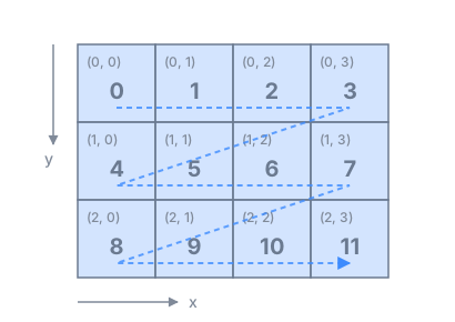
Tile ids on a 2-D grid with axes (y, x) and 3 × 4 tiles: \(k = 4\, t_y + t_x\).#
The tile id in formulas
At a given level, with the origin \(o_a\), the tile size \(s_a\) and the number of tiles along axis \(a\), \(n_a\), as in Grid and tiles, the tile containing a position \(p\) has, along each axis \(a\), the coordinate
With the axes \(a_1, \dots, a_d\) in the order declared in the metadata, its id is
i.e. each coordinate is multiplied by the number of tiles along all the axes that come after it. For the usual axis orders:
With \(N = \prod_a n_a\) tiles, \(0 \le k < N\).
One could instead order the tiles by Morton code (Z-order), which keeps tiles that are close in space close in the order. This is not done in this version and is left for future versions.
Priority#
Every point \(i\) MUST have a uniformly sampled random value \(p_i \in [0, 1)\), termed priority, adapted from the continuous level of detail of van Oosterom et al., 2022 and Schütz et al., 2019. It is drawn once when the points are written and MUST be stored with them, as a column (see Columns). Any uniform random generator may be used, and \(p\) may be derived from a hash of the point. The priority is fixed: it defines which points are in which level, and the order of the rows inside a tile, in both orders of the points. When an element that already has \(p\) is indexed again (another tile size, the other format, a new feature-major table), writers MUST keep its \(p\), so that the levels hold the same points.
\(p\) MUST be of the form \(k / 2^{b}\), with \(k\) an integer in \([0, 2^{b})\) and \(b\) the precision declared
in the metadata (p_bits, see Columns): it is stored as \(k\), and comparisons with the
fractions \(P^{(l)}\) are then exact. Writers SHOULD draw \(k\) directly as a random integer. Drawing a real
number and rounding it is a common mistake: for instance, a value \(u = 0.99999999\) drawn in \([0, 1)\) in
double precision becomes exactly 1 when rounded to single precision (float32 has 24 bits of precision,
so every \(u \ge 1 - 2^{-25}\) rounds to 1), and \(p = 1\) belongs to no level, since level 0 holds the
points with \(p < P^{(0)} = 1\). In the same way, rounding can move a value across a fraction \(P^{(l)}\),
so that the band of a point computed before and after rounding disagree.
Levels and bands#
Every point belongs to exactly one band \(l \in \{0, \dots, L\}\), \(L \ge 0\), given by its \(p\) and by fractions \(1 = P^{(0)} > P^{(1)} > \dots > P^{(L)}\) (see Sampling):
With \(L = 0\) there is a single band, with all the points; bands \(1, \dots, L\) MAY be present. The comparisons are strict: a point with \(p = P^{(l)}\) exactly is not in level \(l\). The tiles of band \(l\) are those of the grid of level \(l\). Level \(l\) is the union of the bands \(L, L - 1, \dots, l\), the points with \(p < P^{(l)}\); level 0 holds all the points.
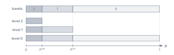
A level is the union of its band and all coarser bands.#
This is the priority-band (continuous level of detail) organization of van Oosterom et al., 2022, with discrete bands on a grid.
Tile-major order and feature-major order#
An order is a table with all the points and all their columns, sorted in a given way. The points are written in exactly one tile-major order and in zero, one or more feature-major orders, one per feature column chosen by the writer and named in the metadata:
tile-major order, which MUST be written: sorted by band (coarsest first, see Levels and bands), then by tile id on the grid of the band, then by \(p\);
feature-major order, optional, for a given feature column named in the metadata: sorted by feature, then by band, then by tile id, then by \(p\). The feature is a categorical column chosen when writing: for spatial transcriptomics, usually the gene id. A writer MAY choose several feature columns, for instance the gene id and the cell type, each with its own feature-major table; it SHOULD choose at most one, the column used most often to select points, for the best performance at the lowest storage cost.
Both orders hold exactly the same points at every level; only the order of the rows differs, so a client gets the same result from either, at a different cost. Since each order is sorted by band, coarsest first (see Levels and bands):
each point is stored once per order: the levels need no extra storage (up to 1.33× in 2-D if each level were a table of its own);
going to a finer level reads only the next band; the points already loaded stay valid;
with the rows of each tile sorted by \(p\), a client can stop reading at any budget \(b\), not only at the \(P^{(l)}\) of the levels (see Reading with a budget).
The two orders answer two different questions with a contiguous range of rows:
Tile-major order: which points are in this region? The points of a tile are one row range, whatever their gene. A client showing the region reads the tiles in view.
Feature-major order: where are the points of this gene? The points of a gene are one row range; inside it, the points of each band are one range, and inside a band the points of each tile. A client showing a few genes reads only their points.
A client looking for the points of a feature uses the feature-major table of that column if there is one. Otherwise it falls back to the tile-major table, as for any other column: it reads every point of the tiles in view and discards the other features, so the cost grows with all the points in view, not with the points of the feature; zoomed out, this can be most of the data. The price of the feature-major table is a second table of the points. Per-tile statistics (e.g. which features a tile contains, or how many points of each) could let a client skip tiles without the feature it shows and improve performance; they are out of scope for this RFC.
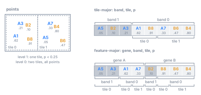
The two orders, as bands. Each table holds every point once, in the band of the coarsest level that holds it: band 1 is level 1 (\(p < 0.25\)), and both bands together are level 0.#
Sampling#
Sampling chooses the fractions \(P^{(l)}\) of the levels (see Levels and bands). The fractions are fixed rates: they do not depend on how many points the tiles hold, and the same \(P^{(l)}\) applies to all the points, whatever their feature, and to both orders. Level \(l\) keeps the points with \(p < P^{(l)}\).
By default, the fraction of a level is the ratio of the tile volumes (areas in 2-D) of level 0 and of that level:
A tile of level \(l\) then covers \(V^{(l)} / V^{(0)}\) tiles of level 0 and keeps that fraction of their points, so it holds on average as many points as a tile of level 0 in the same region, whatever axes were merged. With the merge rule, each level divides the fraction by 2 per merged axis: \(1 / 2^d\) per level when all \(d\) axes are merged (1/4 in 2-D, 1/8 in 3-D), more when only some are. A writer MAY choose any other rates, as long as they strictly decrease with \(l\). When a level keeps the grid of the level below, the tile volume does not change and the default would keep the same fraction; the writer then chooses the rates, e.g. \(1/2^d\) per level. Dense regions stay denser than sparse ones: the sample is density-preserving.
Because \(p\) is uniform, keeping the points with \(p < P^{(l)}\) keeps each point with probability \(P^{(l)}\), independently of the others.
The \(P^{(l)}\) of every level present, including \(P^{(0)} = 1\), MUST be given in the metadata (see Metadata); a reader uses the values of the metadata, whatever rates the writer chose.
Sampling in formulas
A tile of level \(l\) with volume \(V^{(l)}\) (area in 2-D) in a region of density \(\rho\) holds on average
points. With the default rates \(P^{(l)} = V^{(0)} / V^{(l)}\) the two factors cancel, and \(n^{(l)} = \rho\, V^{(0)} = n^{(0)}\) at every level. With the merge rule and all \(d\) axes merged at every level, \(V^{(l)} = 2^{d\,l}\, V^{(0)}\) and \(P^{(l)} = 2^{-d\,l}\). For example, in 2-D with tiles of 10 × 10 at level 0 and of 40 × 40 at level 2, a tile of level 2 covers 16 tiles of level 0 and keeps 1 point in 16.
A client MAY support only level 0 and ignore the sampled levels, and show zoomed-out views with other strategies, such as aggregation (see RFC 4).
Choosing the tile size and the rates#
The levels and the tiles let a client read only a part of the data: the tiles in view, at a level coarse enough for the view. This works well only if the tile size and the rates suit the data and each other. There is no parameter for this in the format: the number of points per tile at each level, \(n^{(l)}\), follows from the density of the points, the tile size and the rates (see Sampling), and guides the choice of the two.
A good target is the number of points a client can comfortably load and display at once from one tile, for now about 10,000, while this RFC is a draft; it will be adjusted from user feedback. The reasoning: with the coordinates and a feature code, about 16 bytes per point, a tile is about 160 kB before compression, a comfortable size for one request, and a view of 4 × 4 tiles shows about 160,000 points, which a browser renders easily. The target is not stored in the metadata and is not a cap: level 0 holds all the points, and a tile may hold any number of them.
The tile size of level 0 SHOULD be chosen for the typical tile, not for the densest one: the median number of points per non-empty tile of level 0 SHOULD be about the target, between 5,000 and 20,000, which usually gives \(10^4\) to \(10^5\) tiles at level 0. If the typical region has \(\rho\) points per unit of area (2-D) or volume (3-D), the tile size along each of the \(d\) axes is about
This estimate assumes that the tiles are isotropic. In practice, a writer can pick a tile size, compute the median number of points of the non-empty tiles, and adjust. Real data are uneven: sizing the tiles for the densest tile makes the typical tile far too small. In two 10x Atera datasets (740 million and 1.2 billion transcripts), tiles sized so that the densest tile holds 10,000 points were 7–9 µm wide, with a median of 200–350 points per tile and 0.8 to 1.9 million tiles; tiles of 27–35 µm give a median of 6,000–9,000 points and 50,000–120,000 tiles. The densest tiles then hold about 100,000 points, which is not a problem: the rows of a tile are sorted by \(p\), so a client reads only as many of them as its budget allows (see Reading with a budget), and the storage splits large tiles into several row groups or chunks (see Points as a tall table).
With the default rates, \(n^{(l)} = n^{(0)}\): the tiles then hold about the same number of points at every level (see Sampling). What is stored per tile is a band, a part of its level: band \(l\) holds a fraction \(1 - P^{(l+1)} / P^{(l)}\) of the level-\(l\) points of the tile (3/4 in 2-D with all axes merged).
The cost of a view stays about the same as the client zooms in and out, plus one cost of the bands: to show a small region at full detail, a client also needs the points of the coarser bands in that region. These are stored in the larger tiles of the coarser levels, so the client reads those larger tiles and discards the points outside the view.
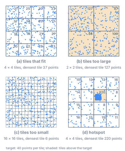
The tile size of level 0 for a target of 40 points per tile, on 400 points.#
The figure shows the edge cases:
(a) Tiles that fit: the typical tile holds about the target number of points.
(b) Tiles too large: the tiles of level 0 hold far more points than the target. Level 0 is not sampled, but a client zoomed in does not have to load a whole tile: its rows are sorted by \(p\), so the first rows are a fair sample of it (see Reading with a budget), and the storage can split it into several row groups or chunks (see Points as a tall table). The cost is coarser spatial selection: a client still reads tiles that are only partly in view. A finer grid is better.
(c) Tiles too small: many tiles with few points each, so a view needs many small requests and the index is large. With the default rates, each level keeps about as many points per tile as the level below, so the tiles of the coarser levels hold few points too, and a view needs many small requests at every level.
(d) Hotspot: a region much denser than the rest puts many points in a few tiles. A tile size chosen for the hotspot is too small elsewhere, as in (c); one chosen for the rest is too large in the hotspot, as in (b), and handled as in (b): this is why the tile size is chosen for the typical tile. A future extension could address this with an adaptive grid, if the community identifies it as a need.
The grid and the rates are the same for all the features, so a rare feature has few points per tile, and at the coarser levels few or none: in the feature-major table most of its tiles are empty. This is not a problem: an empty tile holds no rows and costs nothing in the feature index, which stores only the non-empty tiles of each feature (see Feature index), and the rows of a feature are contiguous, sorted by band, so a client showing a rare feature reads all its levels, down to level 0, as one contiguous range.
Reading with a budget#
Sometimes a client does not have the resources to read all the points of the tiles in view, even at the right level: for instance with tiles that are too large, as in case (b). Here \(p\) comes into play. With a budget \(b \in (0, 1]\), the client reads only the points with \(p < b\): since \(p\) is uniform, a representative sample of a fraction \(b\) of the points, and since the rows of each tile are sorted by \(p\), the first rows of each tile. The budget is not limited to the fractions \(P^{(l)}\) of the levels: the client reads the coarsest level with \(P^{(l)} \ge b\), the bands coarser than \(l\) in full and band \(l\) up to \(p < b\).
Storage format#
The data model above can be implemented both in Parquet and in Zarr, and this RFC describes both. SpatialData already stores points in Parquet, so the Parquet format is to be interpreted as the default, and the Zarr format as experimental. Whether the Zarr format replaces it or the two coexist will be determined from user feedback and real usage; Zarr would also be more flexible for 3-D shapes (meshes, see RFC 4) and closer to zarr-vectors (see Related work).
The two formats have the same layout and the same metadata; they differ only in how a table of points is stored (Parquet files or a Zarr dataframe), and Parquet adds one file of its own, the Parquet sidecar (see Metadata). The offsets are Zarr arrays in both formats.
The format is self-contained: compatible with the way OME-NGFF stores coordinate systems, but usable on its own, even outside an OME-Zarr store, because its metadata is defined as a Zarr convention. Compatible means that this storage of points could in the future be proposed as an OME-NGFF extension, with the extensibility mechanism of NGFF RFC-8, and later, through an NGFF RFC, as part of the OME-NGFF specification. This is not a goal for now: for the time being this specification remains part of SpatialData, and is neither an official OME-NGFF extension nor OME-NGFF compliant.
The spatial index is optional (see Overview). Without it, an element is stored as today (see Compatibility). With it, the metadata declares which parts are present (see Metadata).
Points as a tall table#
In both formats, each table of points is a tall table: one row per point, one column per attribute. The tile index and the feature index address rows (see Tile index, Feature index), so how the rows are grouped into row groups (Parquet) or chunks (Zarr) does not change the index: a row group or a chunk may hold several small tiles, and a large tile may span several. A reader maps a range of rows to the row groups or chunks that overlap it: in Zarr, with chunk length \(c\), the rows \([\,a, b\,)\) are in the chunks \(\lfloor a / c \rfloor, \dots, \lfloor (b - 1) / c \rfloor\); in Parquet, through the part files of the table (see Metadata) and the row counts in their footers. A range of rows MAY span several row groups, chunks, part files or shards, and readers MUST support it.
The row groups and chunks are a choice of the writer, guided by two costs. Each row group or chunk is one unit of reading: a tile smaller than it costs the read of its neighbours, so they should not be much larger than the tiles in view. Each row group also adds an entry, per column, to the footer of its Parquet file, which a reader parses before it reads any row of that file: tiny row groups make the footers large (with one row group of about 10,000 rows per tile, 740 million points give 67,000 row groups and footers of about 2.6 MB per part file). Recommendations:
Parquet writers SHOULD use row groups of about 100,000 to 1,000,000 rows (a few MB compressed), each holding several consecutive tiles, and SHOULD split a larger tile into several row groups. A row group SHOULD start at the start of a tile. In the feature-major table, the same with the rows of one feature in one band.
Parquet writers SHOULD start a new part file only at the start of a tile of a band (tile-major table) or of a feature in a band (feature-major table), so that the rows of a tile are in a single file.
Zarr writers SHOULD choose a chunk length of the same order as the rows of a typical tile, and SHOULD store the chunks in shards (Zarr sharding codec), e.g. of a few million rows: with chunks of one tile and no shards, a table has one object per chunk and per column (about 74,000 per column for 740 million points). Writers MUST NOT write the same shard concurrently from several processes or threads without coordination: a partial write of a shard rewrites the whole shard.
Another option in Zarr is rectilinear chunk grids, an experimental Zarr feature that allows chunks of different sizes along an array: each tile would then be one chunk of its own size.
A spatial index without a spatial subdivision is a special case of this format, not a separate one: a grid with a single tile covering all the points, the same at every level (see Grid and tiles). Each band is then one range of rows sorted by \(p\), so any first rows of a band are a uniform sample of it, which a reader can load progressively.
File layout#
The two formats have the same layout; only the tables differ (Parquet files or a Zarr dataframe, see Columns):
points/<name>/
├── zarr.json                      # attrs incl. spatial_index
├── spatial_index.parquet.json     # Parquet only: the Parquet sidecar
├── spatial/                       # tile-major order, all bands
│   ├── points.parquet/            # Parquet: part files, listed in the sidecar
│   │   ├── part.000000000000.parquet
│   │   └── …
│   ├── points/                    # Zarr instead: df: convention
│   │   ├── columns                # ["x", "y", "z", "gene", "__spatialdata_p__", …]
│   │   ├── column_0               # x
│   │   ├── …
│   │   └── column_3/              # gene, enum: convention (codes, enum_values)
│   └── tile_offsets/              # the tile index of each band: 0, 1, … (Zarr arrays)
└── feature/                       # optional: one feature-major table per entry of feature_keys
    └── gene/
        ├── points.parquet/        # Parquet; or points/ (Zarr)
        └── tile_offsets/          # the feature index of each band: 0, 1, … (Zarr groups)
In Zarr, the offsets sit next to the dataframe, not inside it: the df: convention requires all the
members of the group to be columns of the same length. The offsets SHOULD be chunked so that a lookup
reads one small chunk, e.g. 65,536 entries.
Metadata#
The metadata is a Zarr convention, spatial_index, in the zarr.json of the Zarr group of the points
element, next to the existing attributes of the element, the same in both formats. It is registered in
zarr_conventions with its name and the URL of this specification; the uuid and a JSON schema are
optional and will be added when the convention is released. levels lists the levels present, level 0
first, each with its grid and its fraction:
{
  "zarr_conventions": [
    {
      "name": "spatial_index",
      "spec_url": "https://spatialdata-spec.scverse.org/rfcs/0003-tiled-points.html",
      "description": "Tiled and multiscale points"
    }
  ],
  "spatial_index": {
    "version": "0.1.0-draft",
    "axes": ["x", "y", "z"],
    "feature_keys": ["gene"],
    "p_bits": 16,
    "levels": [
      {
        "origin": [0.0, 0.0, 0.0],
        "tile_size": [35.0, 35.0, 40.0],
        "grid_shape": [280, 170, 1],
        "P": 1.0
      },
      {
        "origin": [0.0, 0.0, 0.0],
        "tile_size": [70.0, 70.0, 40.0],
        "grid_shape": [140, 85, 1],
        "P": 0.25
      }
    ],
    "parquet": "spatial_index.parquet.json"
  }
}
version is the version of this specification that the element follows; it MUST be given, so that
readers can tell future versions (e.g. with tiles in Morton order) apart. While this RFC is a draft,
the version carries the suffix -draft. Following the versioning of Zarr conventions, a released
version will also be referenced by a spec_url (and schema_url) pinned to that version, e.g. a
tagged URL. axes MUST list all the spatial axes of the element (see Grid and tiles).
levels[l] gives the grid of level \(l\): origin, tile_size and grid_shape (the number of tiles
\(n_a\) along each axis, here a single tile along z). P is the fraction \(P^{(l)}\) of the level (here 1/4,
the default in 2-D tiles), the same for both orders: level \(l\) holds the points whose value of \(p\) is
below P. The P of level 0 MUST be 1: level 0 holds all the points. p_bits is the precision of \(p\)
(see Columns). feature_keys lists the feature columns, each with its own feature-major
table (see File layout); it is empty if there is none. The tile-major table is always
present.
parquet is present only in the Parquet format: the path, relative to the element, of the Parquet
sidecar, a JSON file that holds what exists only because the Parquet tables are split into several
files:
{
  "tables": {
    "spatial": {
      "files": ["spatial/points.parquet/part.000000000000.parquet",
                "spatial/points.parquet/part.000020000564.parquet", "…"],
      "first_row": [0, 20000564, "…", 740442119]
    },
    "feature/gene": {
      "files": ["feature/gene/points.parquet/part.000000000000.parquet", "…"],
      "first_row": [0, "…", 740442119],
      "categories": ["ACTA2", "CD3E", "…"]
    }
  }
}
filesMUST list the part files of each table, in order, relative to the element: the rows of the table are the rows of these files, one file after the other. Readers MUST NOT rely on the order in which a directory lists the files, and writers SHOULD zero-pad the numbers in the file names (as above), so that tools that list and sort the directory read the files in the same order.first_row[i]is the first row offiles[i]in the table, and the last entry is the number of rows of the table (len(first_row) == len(files) + 1). A reader finds the file that holds a row from it, and opens only the footers of the files it reads.categories(feature-major tables): the global category list of the feature column, in the order of the codes of the feature index (see Feature index). In Zarr the global list is theenum_valuesof the feature column, so it needs no sidecar.
The sidecar is kept out of zarr.json for two reasons: it grows with the number of part files (about 45
bytes per file, plus the categories), while spatial_index stays small, and keeping it apart makes clear
which parts of the format are specific to Parquet. With part files of millions of rows, it is a few
kilobytes for most datasets.
Columns#
x,y,z: float32, absolute, in the element’s coordinate system. (Spacing of float32 at 10 cm in µm units is about 8 nm, well below localization error.)Feature: integer codes with the category list stored once. In Zarr, the column follows the
enum:convention: the arrayscodesandenum_values, the categories; the number of features is the length ofenum_values. In Parquet, a dictionary-encoded column. Parquet stores the dictionary of a column once per row group, so the dictionary of a row group SHOULD hold only the categories present in that row group, in any order: with tens of thousands of features, a full dictionary in every row group dominates the size of the table (9.3 GB of 23 GB in a test with 27,000 genes and one row group per tile). The codes inside a row group are then local to it; the codes of the feature index refer to the global list of the Parquet sidecar. Writers SHOULD keep the pandas metadata in the schema of the Parquet files, so that readers such as dask read the column as a categorical (the per-row-group dictionaries are unified when reading).\(p\): in the column
__spatialdata_p__, a name reserved by SpatialData, the same in every element, stored as an unsigned integer \(k\), with \(p = k / 2^{b}\) and \(b\) =p_bitsof the metadata: uint16 for \(b = 16\) (recommended), uint32 for \(b = 24\) or \(32\) (see Priority). The levels need \(P^{(L)} \ge 2^{4 - b}\), so that the coarsest level still holds a fraction close to \(P^{(L)}\): with \(b = 16\) and the default rates in 2-D, at most 6 levels besides level 0; more levels need \(b = 24\). Ties between equal values are harmless: levels compare \(p\) with \(P^{(l)}\), and ties may be in any order inside a tile.Any other columns, unchanged. An identifier column of the points (e.g.
transcript_id) is not needed by the index, and writers MAY drop it: points are usually not annotated by a table, and their only relationship, being within a cell, is either computed when needed (a spatial join) or stored as a column of the points. Sorting by tile also removes most of the compression of a sequential identifier (3.8 GB in the test above).
In Zarr, each table of points is a dataframe following the
df: convention: one 1-D array, or a group
read as one, such as an enum: column, per column, all of the same length.
Order of the columns#
Within a row group, Parquet stores the values column by column: a row group holds
the values of the first column, then those of the second, and so on, in the order of the schema.
The coordinate columns SHOULD come first and next to each other, in the order of axes, followed by
the feature column(s) and __spatialdata_p__, then by the other columns. A client reading the coordinates and the feature
of a tile then reads one contiguous byte range instead of one per column. This is also the column order
of the Celldega profile (PR #423), where it makes
column projection and filtering in the browser more efficient with
parquet-wasm.
In Zarr, each column is an array of its own, all with the same chunk length, so the same chunks of each array hold the same rows: a client reads a tile with one request per column and per chunk that overlaps the tile, whatever the order of the columns. The coordinate and feature columns SHOULD still come first, in the same order as in Parquet.
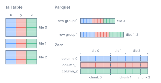
The tiles are row ranges. In Parquet the row groups follow the tiles; in Zarr the chunks have a fixed length and may cut a tile.#
Tile index#
To find the points of a tile, a reader uses the tile index of a band of the tile-major table. Since
the rows of a band are sorted by tile id, the points of each tile are consecutive rows. The index of
band \(l\), which MUST be written, records where each tile starts: an integer array tile_offsets/<l>
(\(O\)) with one entry per tile plus one, for the \(N\) tiles of the grid of level \(l\), in rows of the table.
The points of tile \(k\) in the band are the rows
so tile \(k\) holds \(n_k = O_{k+1} - O_k\) points. An empty tile has \(O_k = O_{k+1}\): it repeats the offset of the next tile, so that the formula holds for every \(k\) and the end of a tile is always the start of the next. The rows of the band are \([\, O_0, O_N \,)\): the range of each band follows from its tile index. A reader reads these rows from the row groups or chunks that overlap them (see Points as a tall table). A client with a budget \(b\) reads the first rows of the tile, until it reaches a row with \(p \ge b\).
The offsets are global row numbers of the table, in both formats. Their integer type MAY be the smallest that holds the number of rows of the table: int32 below \(2^{31}\) rows, int64 otherwise; readers take it from the metadata of the Zarr array. The same holds for the arrays of the feature index.
Feature index#
Each feature-major table MUST have its own feature index, per band. Inside a band the rows of the table
are grouped by feature, then by tile, so the points of feature \(g\) in tile \(k\) are one range of rows.
Most features are absent from most tiles, and the index stores only the non-empty tiles of each
feature, as a CSR (compressed sparse row) structure over the features: a Zarr group
tile_offsets/<l> with three arrays,
tile_offsets/<l>/feature_ptr: [n_features + 1]          # entries of feature g: feature_ptr[g] … feature_ptr[g+1] - 1
tile_offsets/<l>/tile_ids:    [nnz]                     # the non-empty tiles of each feature, increasing
tile_offsets/<l>/row_offsets: [nnz + n_features]        # their first row, + the end of the feature in the band
For feature \(g\), with \(a\) = feature_ptr[g] and \(e\) = feature_ptr[g+1], the non-empty tiles are
tile_ids[a:e], and the \(j\)-th of them holds the rows
[row_offsets[a + g + j], row_offsets[a + g + j + 1]); the last entry of the feature,
row_offsets[e + g], is the end of its rows in the band. This extra end entry plays the role of the
repeated offsets of the tile index: the end of a tile is the start of the next one, and the end of the
last one is given explicitly, so that every non-empty tile is one range found in one array. A feature
without points in band \(l\) has no entries in tile_ids and a single entry in row_offsets: the row where
its range would start. With it, the rows of feature \(g\) in band \(l\) are always
[row_offsets[a + g], row_offsets[e + g]), and, since the table is sorted by feature then band
(coarsest first), the rows of feature \(g\) at level \(l\) (bands \(L, \dots, l\)) are one range, from the
start of \(g\) in band \(L\) to the end of \(g\) in band \(l\).
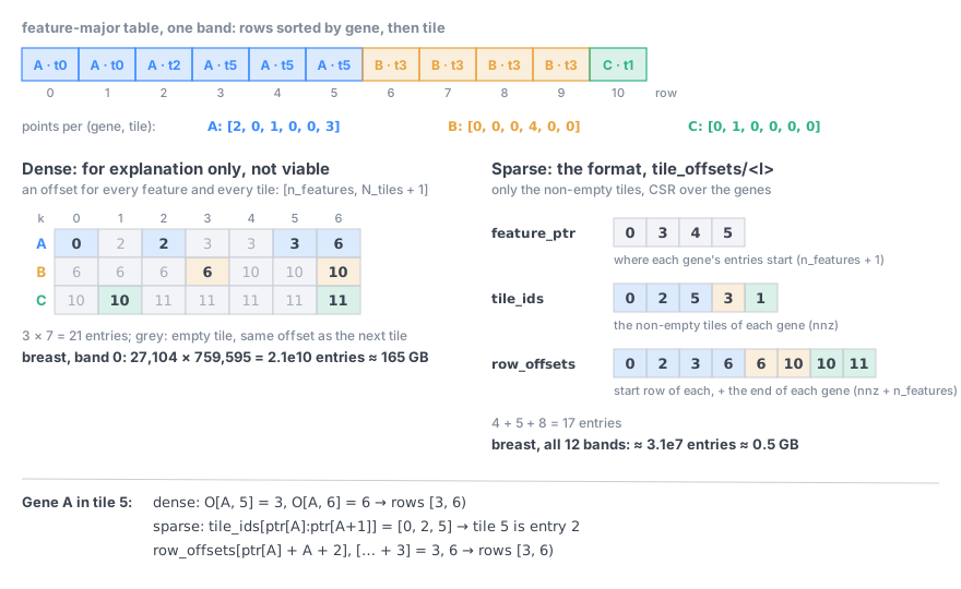
The feature index of one band. Left, for explanation only, a dense matrix with an offset for every feature and every tile, the end of each tile being the start of the next. It is not part of the format: it does not scale to whole-transcriptome panels (27,104 genes on a grid of 760,000 tiles would be \(2 \cdot 10^{10}\) entries, about 165 GB, for one band). Right, the format: only the non-empty tiles of each feature.#
The codes \(g\) are the positions of the features in the global category list: the enum_values of the
feature column in Zarr, the categories of the Parquet sidecar in Parquet. In the example of the orders
figure (see Tile-major order and feature-major order),
with bands 1 and 0 and the 2 tiles of level 0, band 1 has feature_ptr [0, 1, 2], tile_ids [0, 0] and
row_offsets [0, 2, 4, 5] (gene A: tile 0, rows 0 to 2; gene B: tile 0, rows 4 to 5), and band 0 has
feature_ptr [0, 2, 4], tile_ids [0, 1, 0, 1] and row_offsets [2, 3, 4, 5, 6, 8] (gene A: rows 2 to 3
in tile 0 and 3 to 4 in tile 1; gene B: 5 to 6 and 6 to 8). Level 1 of gene A is rows
\([\,0, 2\,)\) and level 0 rows \([\,0, 4\,)\).
The index has about one entry per non-empty pair of feature and tile: in a test with 740 million points, 27,104 genes and 760,000 tiles, 0.5 GB for all the bands.
TODO(Luca): Ilan suggests writing both orders by default, configurable; the proposal said “recommended but optional”. Pending his answer on the Google Doc comment (transcripts or cell matrix?).
Reading#
A client chooses a budget from the number of points in view, counted from the offsets without reading any point, then reads the bands from the coarsest one, from the feature-major table if it shows only some features and the table exists, otherwise from the tile-major table:
n = count_in_view(view, selection)                  # from the offsets, see below
b = min(1, max_points / n)                          # the budget, see "Reading with a budget"
l = coarsest level with P(l) >= b
if selection.features and selection.feature_key in feature_keys:
    for band in range(L, l - 1, -1):                # feature index of that table
        for g in selection.features:
            for k in non_empty_tiles(g, band) ∩ tiles_intersecting(view, level=band):
                yield prefix(rows_of(g, k, band), p < b)
else:                                               # tile-major table
    for band in range(L, l - 1, -1):
        for k in tiles_intersecting(view, level=band):
            yield prefix(range(tile_offsets[band][k], tile_offsets[band][k + 1]), p < b)
# then: drop the points outside the view (tiles cross its edges), and, from the
# tile-major table, the points of the features not shown
prefix(rows, p < b): the rows of a tile are sorted by \(p\), so the points with \(p < b\) are its first
rows; a reader finds where they end from the __spatialdata_p__ column of the tile (e.g. by a binary
search). count_in_view sums \(O_{k+1} - O_k\) over the tiles in view, each weighted by the part of the
tile that lies in the view: the tiles of the coarse bands are larger than the view, and counting them
whole overestimates the points in view by orders of magnitude when zoomed in.
Compatibility#
Without
spatial_indexan element is stored as today, and reads as today.An element with
spatial_indexis a new version of the points format (see the versions of SpatialData): it is not readable by older readers, and the tables are underspatial/andfeature/, the same layout in Parquet and in Zarr. A reader that does not use the index can still read the points from the tile-major table: every point once, sorted by band and tile, with the extra column__spatialdata_p__.
Summary#
The terms of this RFC in three layers. The data is always there. The data model and the storage format of the spatial index are optional; the requirements below apply only to an element that has a spatial index.
Layer |
Term |
Requirement |
Section |
|---|---|---|---|
Data |
the points, one row each, with their coordinates, feature and other columns |
always present, as today |
|
Data model |
axes: all the spatial axes of the element |
MUST |
|
origin \(o_a\) and tile size \(s_a\) of level 0, per axis (a single tile along an axis allowed) |
MUST |
||
bands \(0, \dots, L\) (\(L \ge 0\)): band 0 always, bands \(1, \dots, L\); level \(l\) = bands \(L, \dots, l\) |
MAY |
||
grid of every level present, \(0, \dots, L\) |
MUST |
||
grid of each level refines the grid of the next coarser level (recommended recipe: the merge rule) |
MUST |
||
grids get coarser with the level (a level may keep the grid of the level below) |
SHOULD |
||
tile order: C order of the tile ids |
MUST |
||
random value \(p = k / 2^b\) per point, kept when the element is indexed again |
MUST |
||
fraction \(P^{(l)}\) of every level present (\(P^{(0)} = 1\)), a fixed rate (default: ratio of the tile volumes of level 0 and level \(l\); any strictly decreasing rates allowed) |
MUST |
||
tile size for the typical tile (median of level 0 about 5,000 to 20,000 points) |
SHOULD |
||
feature column(s) |
MAY; at most one SHOULD |
||
Storage format |
metadata: |
MUST |
|
Parquet (default) or Zarr (experimental), same layout |
MUST, one of them |
||
Parquet sidecar: part files in order, their first rows, global categories |
MUST, in Parquet |
||
column |
MUST |
||
tile-major table, levels as bands |
MUST |
||
tile index: |
MUST |
||
row groups of 100,000 to 1,000,000 rows, starting at tiles; part files starting at tiles (Parquet); chunks of about a tile, in shards (Zarr) |
SHOULD |
||
per-row-group dictionaries with only the categories present (Parquet) |
SHOULD |
||
feature-major table, one per feature column |
MUST, for each feature column |
||
feature index: sparse (CSR) |
MUST, with a feature-major table |
||
offsets chunked for small reads (e.g. 65,536 entries) |
SHOULD |
||
coordinate and feature columns first |
SHOULD |
||
identifier column of the points |
MAY be dropped |
Implementation#
An experimental implementation of this draft (both formats, reading and writing, a napari-spatialdata reader that loads the points in view) was tested on two 10x Atera datasets of 0.7 and 1.2 billion transcripts; the numbers quoted in this RFC come from it.
TODO: spatialdata (read/write), spatialdata-io (Celldega PR #423), tissue-map-tools (sampling), a viewer (Celldega, Vitessce, TissUUmaps, merfisheyes, spatiato).
Discussion#
Original proposal by Celldega, September 2026.
Open: the TODO notes above; where CSR/CSC belongs (separate spec, Ilan).
References#
P. van Oosterom, S. van Oosterom, H. Liu, R. Thompson, M. Meijers, E. Verbree, “Organizing and visualizing point clouds with continuous levels of detail”, ISPRS Journal of Photogrammetry and Remote Sensing 194 (2022) 119–131, doi:10.1016/j.isprsjprs.2022.10.004 (PDF, open access, CC BY 4.0). The cLoD value of a point is drawn from a continuous distribution through a uniform random number, \(l = F^{-1}(U)\); it is a monotone function of \(U\), so thresholds on the cLoD value are thresholds on a uniform priority, as here. The paper declares no patent and no competing interests.
M. Schütz, K. Krösl, M. Wimmer, “Real-Time Continuous Level of Detail Rendering of Point Clouds”, IEEE VR 2019 (page): a fixed uniform random value per point, to avoid flicker.